Incorporating Preferences is Easy if You Discretize

tl;dr: Nice figures and animations, mostly. Continuous settings can be hard, but matching and moving arbitrary distributions is easier if you discretize.

Discretizing or binning distributions can make computation of a “probability distance” easier, and certain methods compute gradients for free,meaning we can move and account for distributions with low cost and plug in directly with stochastic-gradient, neural network models!

This post is in companion to work myself and collaborators presented at ICLR 2023, see our paper for more technical discussion. This is a more visual and intuitive explanation of that work, and an excuse to make some pretty animations.

Bird’s Eye View

Often our preferences don’t take the form of a single point, but a distribution over some set of outcomes. To start, let’s say our preference takes the form of a univariate distribution over the real line, i.e., the typical assumptions that come with this picture:

Sometimes we’ll have some other preference, or distribution, along with our own:

If they are different, we might want to figure out HOW different, and even moreso find some “middle ground” or some way to reconcile the difference, “pushing” the distributions to be similar.

We could try to measure this difference with some distance measure. If the distributions are nice like these, then we can easily compute continuous measures of distance, such as KL divergence and others. If it’s possible to write out the distributions as functions of the domain, we might try things like integrating over the difference of the functions.

Down to Earth

However if these distributions are less nice, then this problem can be intractable: we don’t have any nice closed form representations that we can do algebra and easy calculus on to directly compute stuff.

Also, we may have many distributions or preferences that we want to understand and unify.

Ok, so what can we do? Well turns out if we discretize, we can make some cool progress!

In some settings this might even be more valuable than working in the continuous space. It could be hard for me to express a preference or measure continuously, but I could say “I think this outcome or set of outcomes is possible with probability “50%”, corresponding to some discrete uniform mass over a discrete area of input space.

An important part of this is that it’s not really discrete, it’s discretized. We are applying a different topology over the input space. If it were fully discrete, the cost to move from one end to another would be the same as moving just one “bin” over.

Distances With Two Distributions

One way to talk about this mathematically is using the Monge cost definition. Without too much detail, moving further away should entail a higher “cost”. If we want to move one distribution to match another, the cost should naturally be higher if it is “further away”.

Let’s take a simple cost, like just counting the number of “bins” away something is. If one distribution was all in the first bin, and we wanted to “move” or “match” it to another that was all in the last bin, we would have to move all of the “mass” over by the number of bins. This is basically the classical Earth Mover’s Distance.

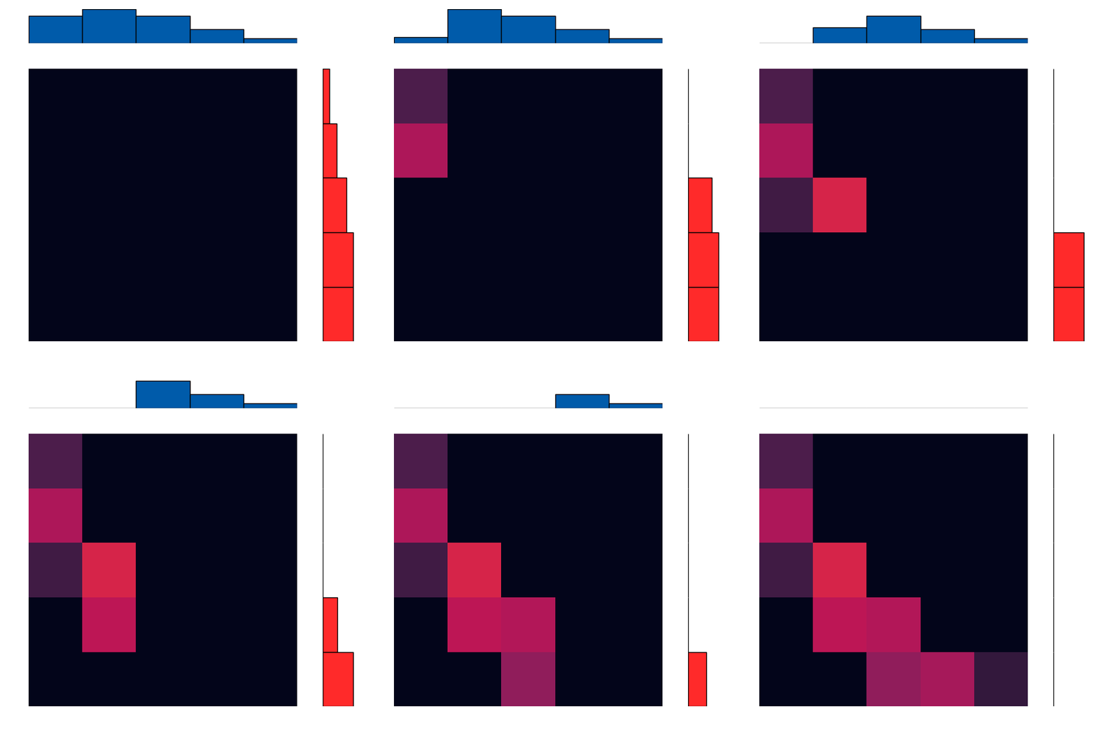
A cool mathematical result that comes out of this is that we can make a single pass over any arbitrary distribution to figure out the cost to make it match another! This ends up being something like a difference match with a carry: at each bin we figure out how much stays and how much moves, and we keep track of how much we have left over. This local operation ends up giving us a global solution.

Another byproduct of this is that the solution we get ends up being a joint distribution, with the marginal distributions equal to the two original distributions!

Here’s a brief animation of the algorithm in action:

With More Distributions

Our ICLR paper focuses on the setting where we may have a larger number of distributions, and we show that everything above extends very naturally and linearly(!) to more distributions.

The above procedure is generalized to find the index of the distribution with the minimum value at any point as we move in axis-aligned steps from the “first” bin at $(0,0,\ldots,0)$ to $(d,d,\ldots,d)$.

Pushing Distributions Together

The super cool part is we can also push those distributions together concurrently, with a “push” direction coming directly from the way we set up the optimization problem to compute the total distance. We didn’t get a chance to explore too much with respect to visualizations for the paper, so here are a few more explorations as we minimize this distance. If you want more technical details, definitely check out the paper, but the tl;dr is that the gradient of the linear optimization problem is exactly the dual variables, and the algorithm we use to compute the distance gives us the dual variables as a byproduct, meaning we have gradient directions from the “forward pass”!

With some fancy setting of learning rates, we can create some very pretty and satisfying animations, that I think help give some intuition about what’s happening.

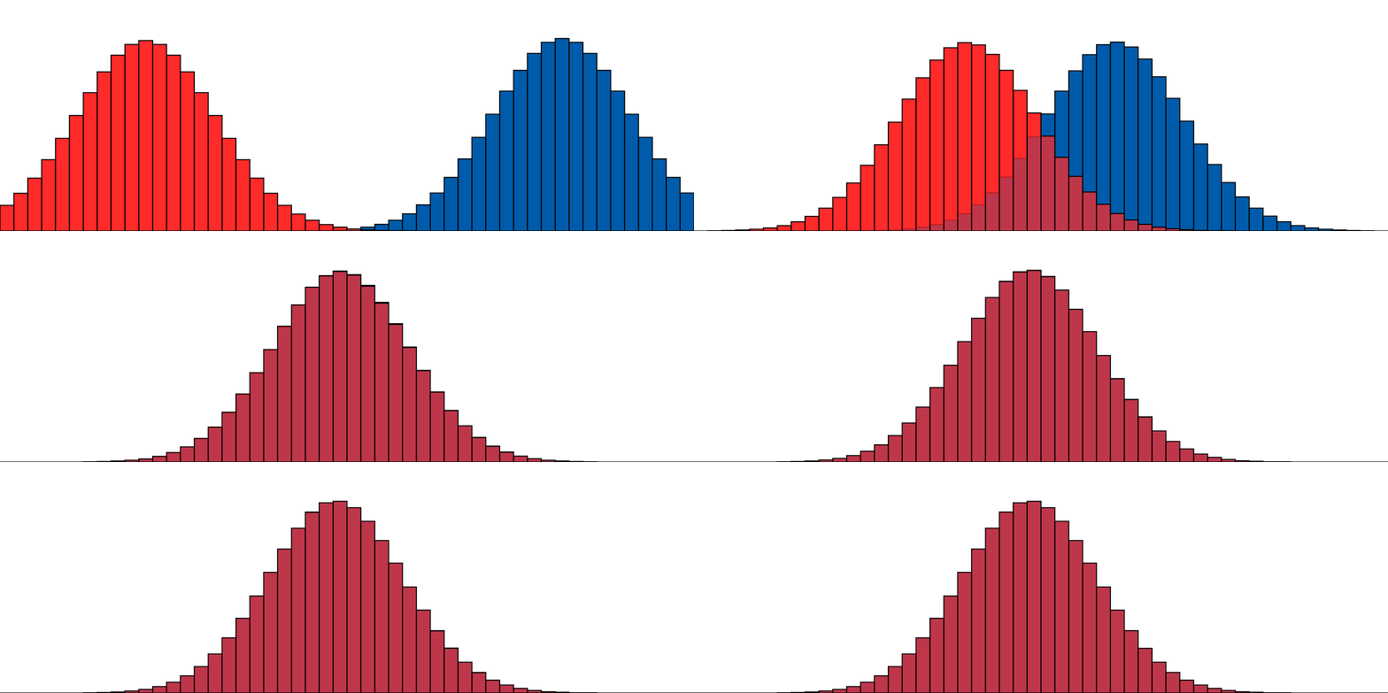
Our simple two-distribution example from above.

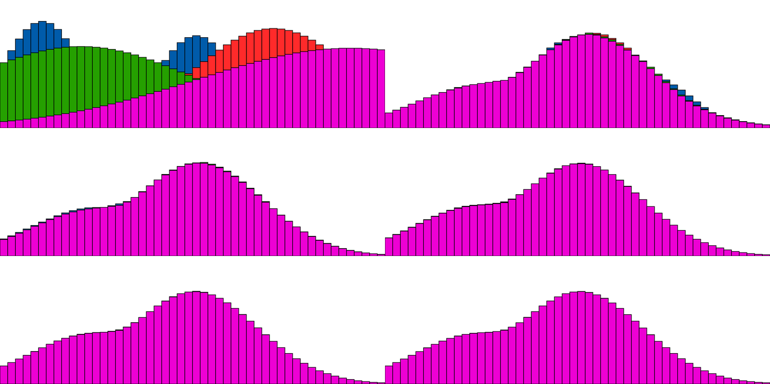
Our more complex one with 4 distributions,

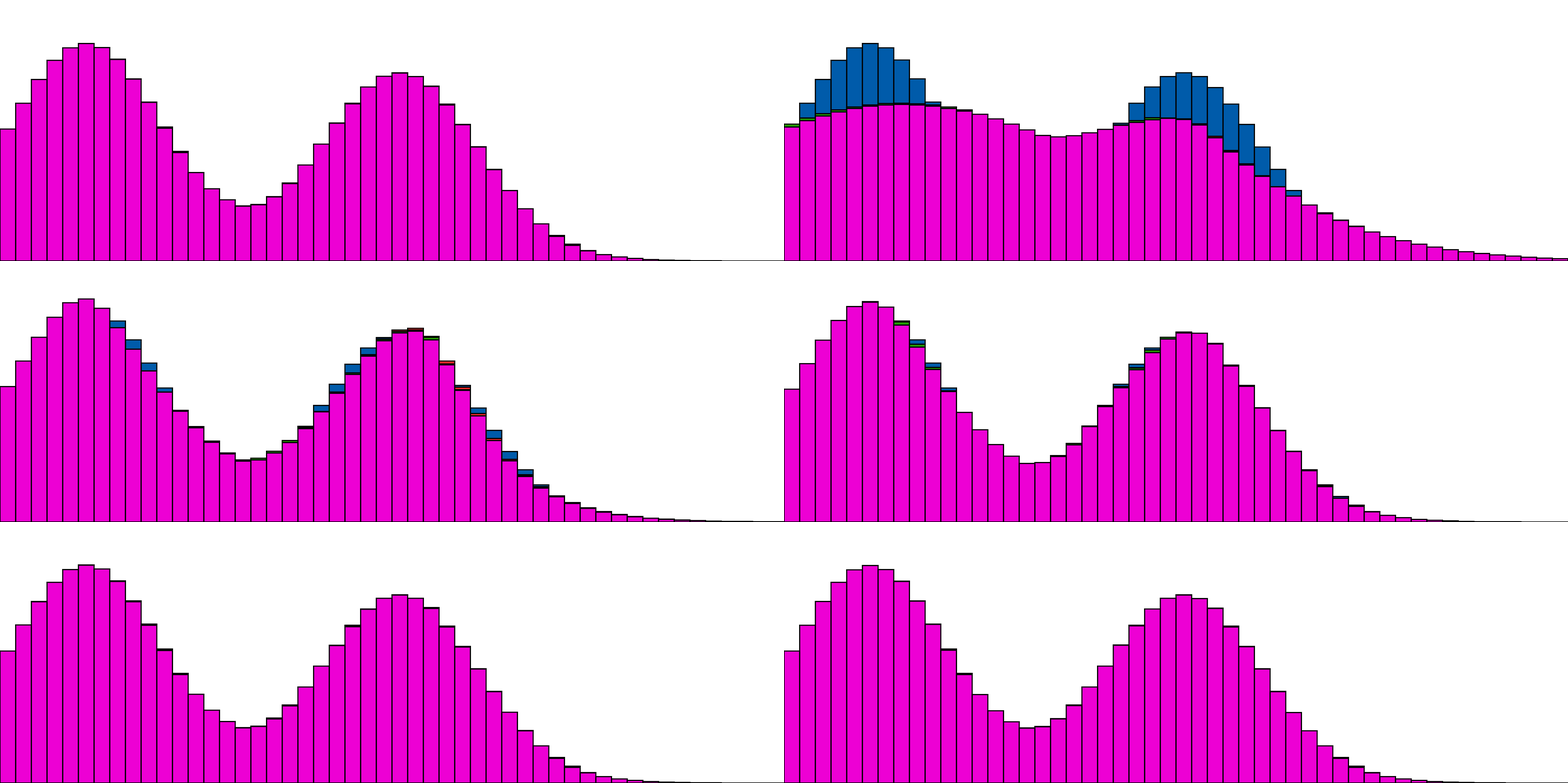
and the same with one distribution as the "target". Here the only change is to disable gradient updates for the target distribution.

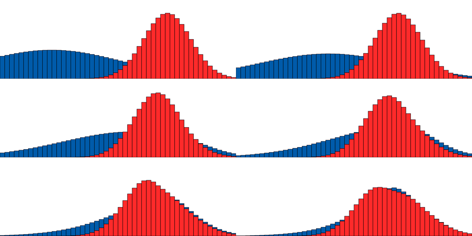
A bit slower, oooh so smooth.

More Practical Applications

Aside from the applications we discuss in the paper, there are a few other places where this could be useful. A big one is in calibration, where we want to ensure that our model’s confidence matches its accuracy. We can use the Earth Mover’s Distance to help inform our training process to push our model towards being well-calibrated. Because the problem is easily extended to many distributions, any types of calibrations, preferences, regulatory requirements, etc. can all be defined, by potentially many different stakeholders, and then reconciled in a single pass!

These can even be private in the federated or distributed learning sense: individual users of a shared learning application can easily compute the distance and gradients locally, and then share the results with a central server to compute the global update.

More Theoretical Questions

As mentioned, an important part of getting some of these pretty animations was selecting the learning rate. In our original work, we used the dual variables as is and applied either a constant learning rate or deferred to the neural network optimizers (i.e., Adam) to determine the gradient step size. However it’s clear that we can choose this in a more informed manner. If we are taking a single step moving mass only locally, we actually know exactly how much mass should be moving and to where: it is porportional to the mass in the current bin and its immediate neighbors.

Can we prove this is linear? I’ve got a feeling it is; there’s definitely a strong connection to isotonic regression, and we can already show empirically that learning rates close to 1 when we normalize the gradient by the amount of mass in the current bin give us fast convergence.

What is the set of solutions this will converge to if all of the distributions are free? Is it some barycenter? If the discretization level goes to infinity, does this approach some continuous result? Our experiments show this works well in the stochastic ML setting, can we identify a theoretical guarantee that this stochastic application is sufficient?

If you’re interested in these questions, or have some of your own, feel free to reach out!

Citation

Ronak Mehta, Jeffery Kline, Vishnu Suresh Lokhande, Glenn Fung, and Vikas Singh. “Efficient Discrete Multi-Marginal Optimal Transport Regularization.” ICLR 2023.

@inproceedings{
mehta2023efficient,
title={Efficient Discrete Multi Marginal Optimal Transport Regularization},
author={Ronak Mehta and Jeffery Kline and Vishnu Suresh Lokhande and Glenn Fung and Vikas Singh},
booktitle={The Eleventh International Conference on Learning Representations },
year={2023},
url={https://openreview.net/forum?id=R98ZfMt-jE}
}