Interpretable by Design - Constraint Sets with Disjoint Limit Points

cart;horse: How can we constrain our models to be interpretable? Convex, linear sets make for more interpretable parameter spaces, and the simplex and the Birkhoff Polytope are great examples of this that have other desirable properties.

An interpretation is something explicit, something discrete, something that compresses, something that summarizes. Our current paradigms do not lend themselves well to this.

We may be able to fine-tune models and interpretations, via approaches built on Provable Guarantees for Model Performance via Mechanistic Interpretability, but in some sense we are fighting an uphill battle against “an uninterpretable base”. In the same way we want to create models that are inherently not capable of deception rather than having to evaluate if an unknown model is deceptive, we should aim to create models that are interpretable by default rather than applying interpretability post-hoc.

Building interpretable architectures and models from scratch with the explicit goal of “simple” explanations isn’t impossible. Interpretability in most cases is compression and discretization, and given both 1) evidence that models can be compressed to effectively one bit per parameter, and 2) now-mature training schemes that work across a wide breadth of model architectures (e.g., Adam), creating networks with these properties is likely possible.

This post is a rough exploration of one direction that seems worth exploring, motivated by some rough set theory and geometry. I tried to keep it short, and there’s an appendix with a bunch of other related ideas and followups.

Unbounded Sets are Hard to Interpret

Let’s say we have a variable or parameter $\theta \in \mathbb{R}$. How do we interpret it?

We can see what the value is and see how far it is from some other number, like 0 or 1.

We can also see how it relates to some other parameter.

But we don’t have any way to interpret it without adding additional points, or by imposing a group or field to give us relevance to the identity elements. Furthermore, the limits of the the parameter space are infinity, and interpretations for “big” numbers have no inherent meaning unless we create additional structure, or talk about relative largeness. Any region of the space looks the same as any other region of the space.

This is also true for real-valued vectors in $\mathbb{R}^n$. We can talk about the relative scale of different dimensions for a given vector, but the limits of the actual values don’t exist, and all regions look the same.

How can we define a parameter space that “looks different” somewhere? One way to think about this question is to think about the limits. The identity elements for whatever operation we want (e.g., 0 or 1) are nice “different” elements, but they aren’t limits. Wouldn’t it be easier to interpret if we could “saturate” in some way? Big numbers tell us something relative to others, but there could exist an even bigger number!

Interpretation needs a limit.

Compact Sets

If we want limit points to be in our set we need it to be closed, and if we want to be able to reach or at least measure those limit points we need the set to be bounded. For subsets of $\mathbb{R}^n$, closed and bounded sets are compact.

Let’s restrict ourselves to the obvious bounded and closed single-dimensional set, $[0,1]$.

Now we have a compact set, with a subset $(0,1)$ that is homeomorphic to $\mathbb{R}$, important because we haven’t lost any representational “power”. The limit points are in the set! This is better. We don’t have a field anymore, but distance to limit points is now a measure, and by checking which limit point we are closer to, we can also discretize to “limiting interpretations”.

We have by-construction-definitions of “signposts” that help tell us where we are, we don’t need to impose them post-hoc. (We can also find ways to build back up to a field and corresponding algebra, but let’s leave that aside for now.)

Care in Higher Dimensions

Notice that in the univariate case of $[0,1]$ our limiting sets are singletons. Depending on how we define our compact set in higher dimensions, this may not be the case, and it matters.

Let’s do the obvious thing and create our compact set as the ball in $\mathbb{R}^n$, the hypersphere plus its interior,

\[B^n_{l_2} := \left\{x \in \mathbb{R}^n\ \middle\vert\ \left(\sum_i x_i^2 \right)^{1/2} \leq 1 \right\}\]

Our limiting points form the set of points defining the surface of the sphere. This set is fully connected. This could be good for some other reasons, but it makes interpretation harder. How do we distinguish between limit points? We again could arbitrarily, post-hoc, assign special values to the limit points at the axis-aligned points, but apriori there’s no reason for these to be special, and optimization schemes will happily move around these points as if nothing interesting is going on around them.

Was this TikZ animation worth the time? Probably not, but it was fun.

In my opinion, this is a large reason why current interpretability is difficult: practical instantiations of $l_2$  norm restrictions tend to have some random mix of “basis-preferring mechanisms”. In ML, this often takes the form of uniform initialization, diagonalized initialization, diagonal Hessian approximations, independence, etc. Without additional structure, interpretations are then arbitrary, equally indistinguishable points that we now need to impose additional structure on.

Interpretations Are Disjoint Limit Sets

The most naturally interpretable spaces are compact sets with disjoint limit sets. There are still a bunch of sets here, which should we choose?

There are some properties we might want that can help reduce the set of possibilities. However we might not want to impose any more structure than necessary, to ensure we are still able to express a large number of different types of objects and functions.

Convexity. We’re probably going to want to search over or optimize over the set, and if its convex that helps a lot. There are many different convex sets, how might we choose among them? Keeping in mind that we’d like disjoint limit sets, what makes the most sense? If we have a limit set 

$A$ and a limit set $B$, then a convex set $C$ must be one where

\[\alpha\cdot a + (1-\alpha)\cdot b \in C,\ \ \forall a \in A,\ b\in B,\ \alpha \in [0,1]\]

If the sets are just points or “corners”, then this describes the line that connects those two points. A convex set must include this line. Interestingly, if we take an arbitrary set of points on a hypersphere and connect them via their convex hull, this is the minimal convex set (by volume) that can include these points. This set can also be defined in the simplest way: linearly!

Linearity. Linear convex sets are defined by a series of intersecting halfspaces described by $Ax \leq b$. They are not only simple to represent but also significantly easier to optimize over. It’s likely we’ll that we’ll need to restrict, project, or otherwise operate on this set. Being able to define the set with linear constraints eases these steps.

Regularity. We could choose arbitrary points on the sphere and construct their convex hull, but apriori we might not really know why or how we should bias the distance between points. Can we create a regular, linear, convex set with disjoint limit sets?

Yes! There are many regular, convex polyhedra that satisfy these constraints. Platonic Solids are the set of these in 3-dimensional space. Which of these should we choose?

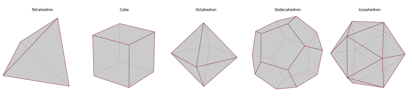
Platonic Solids. Nice.

The $l_1$ and $l_\infty$ Balls

Natural choices might be the the “balls” that are linear. Corresponding to the 3D octahedrons and cubes respectively,

\[B^n_{l_1} := \left\{x \in \mathbb{R}^n\ \middle\vert\ \sum_i |x_i| \leq 1 \right\}\] \[B^n_{l_\infty} := \left\{x \in \mathbb{R}^n\ \middle\vert\ \lim_{p\rightarrow\infty}\left(\sum_i x_i^p\right)^{1/p} \leq 1 \right\}\]

The $l_\infty$ ball can more easily be written as linear constraints similar to the $l_1$ ball to get around the exponential issue. A key difference is that the $l_1$ ball has $2n$ corners, while the hypercube has $2^n$ corners. We can see the hypercube as the convex combination of all possible binary settings of  $n$ bits; this could be interesting as a separate set to optimize over, but an exponential amount of interpretations doesn’t seem tractable to me, at least for now.

Let’s focus on the $l_1$ ball. This is much better if we want to interpret just from the geometry: there’s clearly something special about the corners:

But after that first one the marginal gain is worth it for this one right?

This is great because if we optimize and find a corner, we have two interpretations immediately:

1. What “feature” or “dimension” is relevant. The corners are exactly basis-aligned, so any information flow is completely and only through that dimension.

2. A “direction”. If we are eventually trying to understand positive or negative contributions of particular inputs, or features, or any other objects, we can immediately identify the valence of this particular vector.

Note: our goal here is explicit restriction rather than just regularization: we don’t want to just slap an extra regularizer into our loss: we want to project every vector onto this set before using it downstream. Projection in this case is $O(n \log n)$  because of a necessary sorting, in comparison to projection on the $l_2$ ball which is just $O(n)$. This might not be too bad, but I could imagine this adding up significantly if it needed to happen after every forward pass operation, let alone needing to backpropagate through sorting.

A key issue with this approach is that interior points are still hard to interpret: they are effectively arbitrary vectors, and the only information we can probably get from them is something like “the closest corner”, with some sign information. Additionally, in higher dimensional spaces we don’t really get any natural “dimension reduction”: it’s possible that one of the values is 0 which would reduce to a $n-1$ dimensional ball, but that suffers a similar issue that our  $l_2$ ball surface does: there’s no reason to “stick” there, that 0 element could easily shift or move to be slightly negative or positive.

For these reasons we may want a space where dimension reduction “sticks” in some way.

The Simplex for Elements in $\mathbb{R}^d$

The standard simplex is defined as the set of positive real numbers that sum to 1,

\[\Delta^n :=\ \left\{x_i \in \mathbb{R}^n\ \middle\vert\ \sum x_i = 1\right\}.\]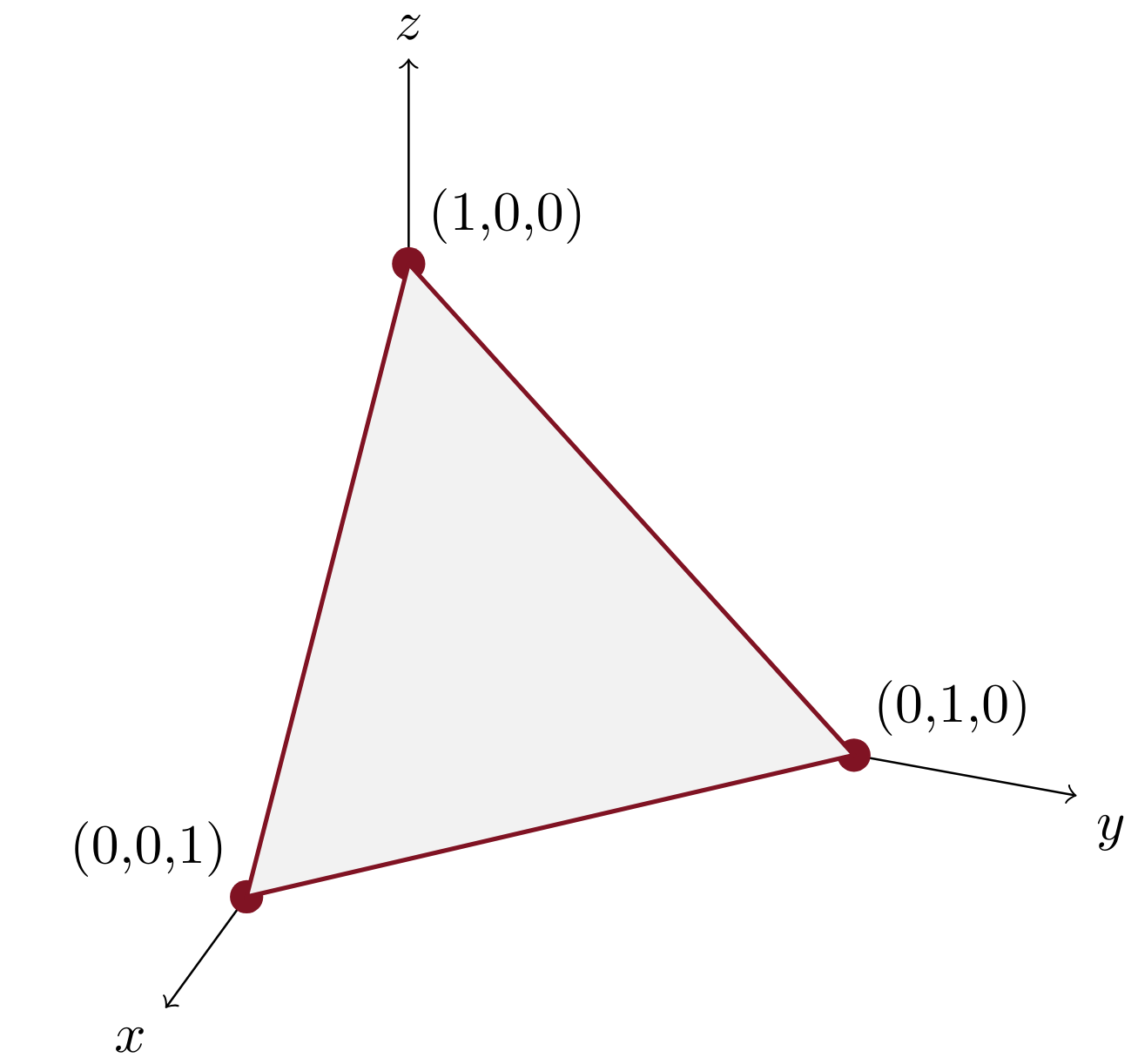

The simplex over the basis vectors in three dimensions.

The simplex has a TON of properties that lend themselves to a more interpretable set.

Natural, Axis-Aligned Bases. The bases where a single element is 1 and the rest are 0 explicitly define our “corners” and correspond directly to “interpretable” points of our set. These are points where all other dimensions are “off”, and the only forward contribution comes from a single dimension. This also means that every element in the simplex is a linear, convex combination of the basis elements.

Probabilistic Interpretations. The standard simplex is also known as the probability simplex. As you can likely see, having everything sum to 1 defines a categorical probability distribution over the dimensions.

Subspaces and Hierarchical Intepretations. The subspace corresponding to a “face” of the simplex is exactly an  $n-1$  dimensional simplex, and corresponds explicitly to the situation where one of the bases is 0. Interpretation here is naturally hierarchical in a linear, composable way.

Sparsity is Encouraged. The points with maximal $l_2$ norm with respect to the ambient space are the corners! The “level sets” with higher $l_2$ norm are closer to subsets of the simplex that have higher sparsity. This means that maximizing  $l_2$  norm while constrained to the simplex increases sparsity.¹

[1]

The simplex, by construction, pushes volume to lie on lower-dimensional subspaces. This is also true of hyperspheres, but there is no bias towards a subspace that is axis-aligned! There may be some interesting combinatorics on the concentration in high dimension here, e.g., the ratio of the surface area to the volume.

A First Pass at Simplex Computations

To map from real numbers to the simplex, there are two options for our map  $\sigma:\mathbb{R}^n \rightarrow \Delta^n$ . The closest point can be computed using:

\[p_{i}=\max\{x_{i}+\delta ,\ 0\}\]

where  $\delta$  satisfies  $\sum_i \max{ x_i + \delta , 0 } = 1$ . This can be computed by sorting  $x_i$  in  $O(n\log n)$  time. As mentioned earlier, this can be bad to have to do during forward or backward passes in a network.

Alternatively, we can use the softmax function:

\[\sigma: \mathbb{R}^n \rightarrow \Delta^n,\quad \sigma(x)_i = \frac{e^{x_i}}{\sum_i e^{x_i}}\]

which we can compute in linear time. Importantly softmax is not idempotent: repeated application of the softmax pushes the vector more and more towards the uniform vector  $[\frac{1}{n},\frac{1}{n},\ldots,\frac{1}{n}]$ . This might not be a good thing: if we want interpretability by being at corners then repeated softmax applications will shrink us away from them.

We can partially address this issue by using another valuable property of the softmax: we can add a temperature which can control how much we bias toward corners of the simplex! Higher temperatures correspond to “more discrete” or more interpretable representations, which may trade-off against other performance metrics in some way.

Notably the softmax operation is fairly easily differentiable: while it has some added cost with computing exponentials, this is much easier to deal with in typical ML pipelines compared to fully discrete operations like sorting.

Practical Issues. Softmax takes more FLOPs to compute compared to ReLU + LayerNorm. It also makes gradients vanish way more easily. There may be other optimization paradigms that make this easier, but this is likely to be a significant barrier to both scaling testing of this approach and convincing others to adopt for production use. There may be ways to solve these problems or the cost could be worth it, but figuring this out will require more work.¹

If we use the softmax, paths on the simplex tend to follow paths of “low entropy”. These look like curves in Euclidean space, but are actually the paths that “try to keep things as similar as possible”.²

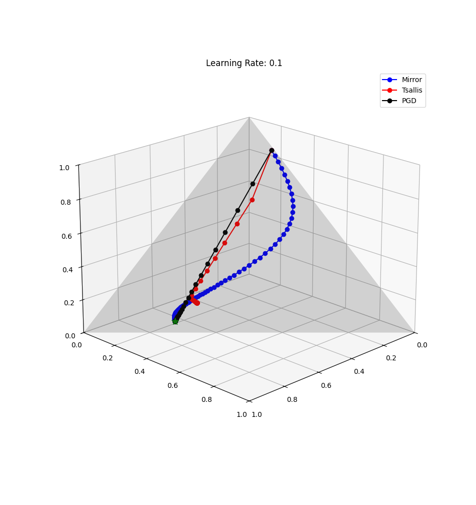
The blue curved path is using Exponential Descent (Mirror Descent on the Simplex), while the other paths represent Euclidean projections and post-hoc regularization.

Optimization also follows subspaces: if there is no optimization pressure to move off of a face, then optimization continues only on that sub-simplex.

Minibatch updates may change which corner we move towards, and eventually there may be pressure to stay “between” a subset. This subset is also a sub-simplex, and we can tune and regularize toward corners.

In this example we start by “feeling” optimization pressure across all corners, but then only for 3 corners; the path then pulls further away from the left-out corner, reducing the effective dimension (more interpretable, sparser).

What’s Next

How do we construct neural-network operations on simplex vectors? We may have to define new operations e.g., constraining a linear layer such that $Wx = y$ for $x,y\in\Delta$. We’re currently exploring some practical implementations of “simplex-constrained neural networks” through a SPAR project. How can we practically constrain existing network architectures, and do we get better “interpretability” by doing so?

Moving from activations to weights in this paradigm requires moving from vectors to matrices. The matrix analog to the simplex is the Birkhoff Polytope.³ The Birkhoff polytope has a ton of properties and theory that naturally extends a lot of the intuitions above to maps.⁴ There’s a lot of cool existing theory to build on here as well.⁵⁶⁷⁸⁹

If anyone would like to chat about these ideas please reach out! I don’t think there are many market incentives to work on this; it’s likely most ideas in alternative architectures will fail and are not worth the R&D that could be used to stay at the frontier. The current academic atmosphere seems unlikely to support research in this direction either: this is a high risk high reward research direction, and unlikely to yield incremental results necessary for success toward paper bean counting.

I’m a little sad that much of safety research has fully pivoted to post-hoc explanations of frontier Shoggoths. I think there’s probably low hanging fruit to grow an easier to understand Shoggoth, even if it’s not with a simplex :).

(An appendix on LessWrong with a bunch of other random ideas that I didn’t have time to organize).

This work is an extension of some ideas I explored during the MATS program.

Footnotes

1. Our SPAR project is exploring some of these ideas, and this $l_2$ observation came directly from experiments done during the project. We’re exploring some ideas with a “Rescaled ReLU”. Our current results suggest practical implementation isn’t easy here, and as always the performance tradeoffs require work to balance. ↩ ↩²

2. Simple here is measured by entropy; [1/2, 1/4, 1/4] is a low entropy state that is an attractor. Claude says related geometric terms here are: median, skeletal elements, and barycentric subdivisions. ↩

3. The Birkhoff polytope is the set of doubly stochastic matrices, i.e., both the rows and columns are all nonnegative and sum to 1. ↩

4. As a preview, the corners of the polytope are the set of permutation matrices, and we can think of interior points as convex combinations of the symmetric group operations over the elements represented by the number of features/dimensions of the input and output spaces. The “faces” or subspaces of the polytope correspond to subgroups of the permutation group. ↩

5. Manifold Optimization Over the Set of Doubly Stochastic Matrices: A Second-Order Geometry. Ahmed Douik, Babak Hassibi. https://arxiv.org/abs/1802.02628 ↩

6. Algebraic and geometric structures inside the Birkhoff polytope. Grzegorz Rajchel-Mieldzioć, Kamil Korzekwa, Zbigniew Puchała, Karol Życzkowski. https://arxiv.org/abs/2101.11288 ↩

7. Probabilistic Permutation Synchronization using the Riemannian Structure of the Birkhoff Polytope. Tolga Birdal, Umut Şimşekli. https://arxiv.org/abs/1904.05814 ↩

8. Beyond the Birkhoff Polytope: Convex Relaxations for Vector Permutation Problems Cong Han Lim, Stephen Wright. https://proceedings.neurips.cc/paper/2014/hash/208e43f0e45c4c78cafadb83d2888cb6-Abstract.html ↩

9. The Birkhoff Polytope is also known as the “transportation polytope”, and there are probably really nice connections to optimal transport theory that we can leverage. ↩