Interpretability As A Science
tl;dr: Knowing the typical or base distribution of a measure is important for interpreting a specific instance of that measure!
Audience: You know some ML math basics, like how losses are typically computed. You are interested in how hypothesis testing can be used to interpret machine learning models, or are confused as to why some particular result you read about isn’t convincing you as much as you hoped.
Abstract
Interpretability of neural network models should be seen through the existing lens of science, and existing hypothesis testing tools will be helpful in “interpreting interpretability”. White-box interpretability of machine learning models is directly analogous to the classical scientific study of real world phenomena. Questions such as “What is this mechanism doing?”, “How well does this mechanism sufficiently explain the outcome?”, “Is this mechanism similar to another?”, and “Does this mechanism have multiple functions?” can all be asked both of the real world and of machine learning models.
Table of Contents
Skip to Scalable Interpretability via Hypothesis Testing if you think you have the background.
- Motivation
- Brief Background: Measuring Loss
- Scalable Interpretability via Hypothesis Testing
- Footnotes
Motivation
There have been a few recent discussions on mechanistic interpretability that set the stage. Though I’ve been sitting on this for some time, these recent public posts reflect a lot of my own motivations for this post.
From How useful is mechanistic interpretability?, it seems like others are also confused and concerned by the value and interpretation of mechanistic interpretability results so far.
Some relevant quotes:
…current work fails to explain much of the performance of models…
…Aim to more directly measure and iterate on key metrics of usefulness for mech interp…
…compare to other methods…
An uncertainty here is whether the lost performance comes from some genuinely different algorithm, vs some clumsiness in our ablations.
(Note that by my definition no interp has ever succeeded on a model trained on a real task, afaik.)…
From Against Almost Every Theory of Impact of Interpretability:
…toy models on cherry-picked problems…
Stephen Casper makes a similar point here: “From an engineer’s perspective, it’s important not to grade different classes of solutions each on different curves.”
Richard Ngo’s comment therein is an underlying theme for this post:
…connect our understanding of neural networks to our understanding of the real world…
Anthropic’s Reflections on Qualitative Research is a strong independent thread providing motivation for the thoughts below, and written up better and faster than I could have or did. This post ends up coming to similar conclusions, albeit from a different angle and with perhaps a bit more precription.
Brief Background: Measuring Loss
Let’s say we have a model $f$ that takes input $x$ and outputs estimate $\hat{y}$, and we compute the correctness of the model against a true $y$ via some loss:
\[l := \left(y - f(x)\right)^2\]or some other distance $d(y, f(x))$ (cross entropy, etc.). If we have some dataset $\cD:= \{x_i,y_i\}_{i=1}^n$, then let
\[\cL(f,\cD) := \sum_{\cD} l_i := \sum_{(x_i,y_i)\in \cD} \left(y_i-f(x_i)\right)^2\]Did We Do Something?
We want to know if we do something to $f$, say $\tf$, if it has done anything to the output we get at $\cL$. “Done anything” is super vague, and I think there’s a lot to unpack there.
A thing we might compute to see if there’s a change could be the difference of the (expected) loss:
\[\cL(f,\cD) - \cL(\tf,\cD)\]After all, we want to know if our change or operation results in a different output, right?
A Representative Pitfall
Let’s say we have 2 “samples” in our “dataset”, and for our original model $f$ they result in losses
\[l(f,1) = 0.4,\ l(f,2) = -0.2,\]and using a typical summation for aggregating the losses, \(\cL(f,\cD) = 0.2\).
Now we take some perturbed or alternate model $\tf$, and it results in losses
\[l(\tf,1) = -2.9,\ l(\tf,2) = 3.1.\]Using the aggregate above we’ll get the same value, and conclude that the change in model did nothing!
Obviously combining losses in this way is not the right thing to do. In classical statistics, this is related to Simpson’s Paradox, where we have correlated samples. We need to account for the fact that each computed loss corresponds to the function taking a specific input: the samples are not interchangeable when comparing measures (stats: random effects).
Great, so the next thing we do is break up the $\cL$ differences by sample and instead look at the aggregate differences:
\[\sum_{i} \left(l(f,i) - l(\tf,i) \right)\]We still have the same problem! The difference has only been distributed, and the above example results in the same conclusion. Ok, but we never look at the simple difference right? We should use the absolute difference, or sometimes equivalently, the squared difference.
\[\sum_{i} \left(l(f,i) - l(\tf,i) \right)^2\]This solves it. With only positive measures of “difference”, the aggregation can’t lead to cancellation, and any differences for each sample will be effectively accounted for in this final measure.
We can also see this effect using linearity of expectations. If we take our distribution over the entire dataset $i\in \cD$.
\[\begin{aligned} \EE_i\left[ \left(l(f,i) - l(\tf,i) \right)^2\right] &= \EE_i \left[l(f,i)^2 - 2l(f,i)l(\tf,i) + l(\tf,i)^2 \right] \\ &= \EE_i \left[l(f,i)^2\right] - 2\EE_i \left[l(f,i)l(\tf,i)\right] + \EE_i \left[l(\tf,i)^2 \right] \end{aligned}\]The expectation (or sum) in the middle term cannot be distributed because the sample $i$ is not independent for both losses. These are exactly those correlated samples that we had to worry about when moving to squared difference! Put another way, we should be careful not to take our means too early!
One Value is Not Enough
But what if our measure is more complicated or has other dynamics? How do we interpret this measure? In this case the measure will be some positive real number, but do we expect it to be zero? Are there small changes that would tell us that the intervention had no effect?
We need some sort of reference to understand how we should interpret the number we get out.
Normalization is often used to obtain a reference:
\[\frac{\cL(f,\cD) - \cL(\tf,\cD)}{\cL(f,\cD)}\]This gives us a scaled distance from the original loss in terms of a known and relevant multiplicative factor. But we still have an issue of understanding the scale: interpretation has not moved further than our original statement of “closer to 0 means less difference.”
Another possible term could be the gain relative to the gain against a random baseline.
\[\frac{\cL(\tf) - \cL(b)}{\cL(f) - \cL(b)} \times 100\%\]As described in the Causal Scrubbing Appendix:
This percentage can exceed 100% or be negative. It is not very meaningful as a fraction, and is rather an arithmetic aid for comparing the magnitude of expected losses under various distributions. However, it is the case that hypotheses with a “% loss recovered” closer to 100% result in predictions that are more consistent with the model.
There are probably variations of this scheme which can be used to deal with these issues, and we can again extend the random effects idea above to help with Simpson’s like cancellation, but it is still one number, and how do we interpret a single number?
Calling back to Anthropic’s Reflections, we need to be able to compare our measure to some reference, and we need to be able to understand the distribution (“Signal of Structure”) of our measure to understand how to interpret a specific outcome.
Scalable Interpretability via Hypothesis Testing
The Causal Scrubbing authors briefly mention that one could look at these measures over the full dataset, i.e., compare the distributions of the random variables $l(f,\cD)$ vs. $l(\tf,\cD)$. This would help us a bit as they mention, but conclude that it would require an explanation of the noise that may be compute-intensive.
I think distributions are necessary for proper interpretability.
The main issue with with a single value is that it does not effectively capture everything that we were wrapping as “explainable” or “not explainable”. And in fact, with a real number we’re really trying to answer “HOW explainable?” “How much is explained by X?” My perspective is that much of interpretability and XAI research is circling around these questions because they aren’t well posed.
But if we harken back to ye olde classical science, I think we can make some progress.
Hypothesis Spaces and Testing
A hypothesis is a claim that we believe might explain some world phenomena. Consider these two hypotheses, one about the real world and one about an arbitrary neural network transformer model:
\[\begin{aligned} H &:\qquad \text{Fruits are healthy.} \\ % \label{hyp:world} \\ H &:\qquad \text{Transformers do induction.} %\label{hyp:ml} \end{aligned}\]We know almost by gut that these are tall claims that are effectively impossible to actually, really prove. But we have intuitions or general beliefs they might be true, because we have evidence for more concrete hypotheses that each themselves provide evidence for these.
But if we actually want to build up to these, and want to formally test and do something to evaluate them, we need to zoom in.
\[\begin{aligned} H &:\qquad \text{Apples have a lot of Vitamin C.} \\ % \label{hyp:world} \\ H &:\qquad \text{The 1.5 and 2.4 attention heads are important for induction.} %\label{hyp:ml} \end{aligned}\]As written, these still both have a number of practical problems for actually doing a proper test. How much is “a lot”? How do we define “important”? How do we measure Vitamin C? How do we measure “important”? If we have multiple measures, which should we choose? An arbitrary test of these hypotheses as stated would be hard to implement, evaluate, and trust.
A good hypothesis is a falsifiable one. Any claim may have some evidence supporting it (its likelihood may be nonzero), but without testing alternative claims to establish a baseline likelihood, we won’t know how much we should update and stop thinking about alternative explanations.
For this reason, classical hypothesis testing requires rigorous definitions of a full experiment, a hypothesis test, including not only the measure and the specific hypothesis, but also the space of hypotheses.
After a measure is chosen to evaluate the hypothesis of interest (e.g., a test statistic), it’s evaluated and compared to other hypotheses within that space: how likely is it to explain the evidence compared to other hypotheses within its class? In the real world example above, what is the space of relative hypotheses? All other fruits? All other foods? Anything for which we can measure Vitamin C? This choice explicitly defines how we can judge “a lot”, and what alternative hypotheses we may be able to now ignore.
Different choices can completely reverse our conclusion to the original vague claim. Apples may have “a lot” of Vitamin C compared to other foods, but may not have “a lot” more compared to other fruits. Similarly for our transformer, are we comparing to a another specific path? Paths with one head from each other layer? All possible head subsets?
These questions lead to the classical hypothesis testing construction where a null hypothesis must be defined as a different element or region of the hypothesis space compared to the claim we wish to test. If we want to compare to oranges, then we need a measure that works for oranges, and we need to measure them. If we want to compare to all fruits, then we need something that works for all fruits. If we want to compare to all other paths through the network, we need our measure to work for all of those paths.
\[\begin{aligned} H_A &:\qquad \text{Apples have \textbf{more} Vitamin C compared to \textbf{other fruits}.} \\ % \label{hyp:worldA} \\ H_0 &:\qquad \text{Apples have the \textbf{same amount or less} Vitamin C compared to \textbf{other fruits}.} \\ % \label{hyp:world0} \\ & & \\ % \nonumber\\ H_A &:\qquad \text{The path through attention heads 1.5 and 2.4 is \textbf{more important}} \\ % \nonumber\\ & \quad\qquad \text{for induction compared to \textbf{any other path}.} \\ % \label{hyp:mlA} \\ H_0 &:\qquad \text{The path through attention heads 1.5 and 2.4 is \textbf{equally or less important}} \\ % \nonumber\\ & \quad\qquad \text{for induction compared to \textbf{any other path}.} % \label{hyp:mlo} \end{aligned}\]Concretely we are now determining if our hypothesis is more likely compared to another (or another group). In these cases, these hypotheses represent the entire set of possible outcomes. If we had a measure, there wouldn’t be an outcome that describes some different hypothesis subsumed here. Classical hypothesis testing gives us this for free by requiring that nulls and alternatives explicitly define corresponding regions of the outcome or measure space, and even describe testing frameworks that ensure the entire space of outcomes is formed by the disjoint union of the two.
From a probabilistic or Bayesian perspective, we’re comparing the likelihood of observing these phenomena among possible “worlds.” Bayes factors and credible intervals can be used in place of significance testing and confidence intervals: we don’t have to go all the way to those scary frequentist $p$-values if we don’t want to.
Unique for the case of machine learning models is that the entire “world” is explicitly defined, and we can actually compute population-level statistics, i.e., all possible activations, for all possible inputs. Obviously computational complexity may limit or restrict full testing in practice, but using such hypothesis testing frameworks allow us to minimally fall back on sample-based statistical testing.
Practical Testing
How do we test a hypothesis once we have one? In the real world case, we cannot know for certain that all apples have more Vitamin C compared to all fruits, but we can collect samples of both and use a measure on those as an estimate of the population measure. We can go collect apples and other fruits directly from our world, and compute some measure that gets at the “amount” of Vitamin C. We can “select” paths through our transformer and compute some measure that gets at the “importance for induction” of that path.
These sample selection procedures are part of the test definition. If we want to say something about the population mean via a sample mean, it is expected that the sample is representative in some form: the individual samples collected are independently and identically distributed. Clearly in the neural network setting, this may not be the case: paths through the network that overlap significantly would obviously have correlated values, and we might want either our measure to reflect this, or to understand this limit as part of the test we construct.
What could these measures look like? There may be multiple ways to measure Vitamin C, and the choice of measure may imply different assumptions about the world. This could include actual data collection methods, like when the end of some titration is decided, or it could include what statistical aggregation and parameters were used, such as sample size, type of mean, or other hyperparameters. The details of the measure chosen are also part of the hypothesis test definition.
If we just “squeezed” the fruits until they stopped dripping, it’s easy to see that this assumes something about where the Vitamin C is, or at least that this process retrieves the same amount of it across differing fruits. In the same way, we should make sure that the metric we choose for evaluating importance for interpretability encodes the assumptions we are actually making about the model.
Evaluating Measures. In the classical case, we typically have an interest in the population mean, taking advantage of efficient properties that allow testing against closed form null distributions. “On average, is there more Vitamin C in apples compared to other fruits?” Just because the observed difference in means is large, does not mean that the population difference may be large as well. The null distribution encodes our prior belief about how the difference would be distributed if there were no differences between the true population means $\mu$.
\[\begin{aligned} H_A &:\qquad C_{apples} > C_{others} &H_A &:\qquad \mu_{apples} > \mu_{others} &H_A &:\qquad \bar{x}_{apples} > \bar{x}_{others} \\ %& %\qquad\qquad\qquad\qquad\qquad\quad \Rightarrow & & \qquad\qquad\qquad\qquad\qquad\quad \Rightarrow & & \nonumber\\ H_0 &:\qquad C_{apples} \leq C_{others} &H_0 &:\qquad \mu_{apples} \leq \mu_{others} &H_0 &:\qquad \bar{x}_{apples} \leq \bar{x}_{others} %\\ \end{aligned}\]In this simple situation the distribution of the difference of the means is well studied and can be tested directly. The expected distribution of this statistic, with many different assumptions about the variance, is known and easily computable: a commonly used tool in a statistician’s toolbox.
Back to Interpretability
Let’s generalize the transformer/induction hypothesis back to our initial example and say we believe that a part of some model or function $f$ is doing some operation $g$. Our hypothesis is that if it is doing that function, we can replace that part of the model with $g$ and the output of the model will not change. Call the model with the replaced module $\tf$. Then we want to test:
\[\begin{aligned} H_A &: \cL(f) = \cL(\tf) \\ H_0 &: \cL(f) \neq \cL(\tf) \end{aligned}\]In this setting, we are explicitly focusing only on a single part of $f$, and determining if it is performing a particular function compared to others. We are not testing if other parts of $f$ are performing that function better. This distinction is critical! These decisions define the hypothesis space, can lead us to different measures, and can lead to different conclusions.
What would it mean for them to not be equal? It’s unlikely we’ll get exact equality if we were to do this in practice, so what would we expect the gap to look like? Well if it that part of the model wasn’t doing $g$, or at least not $g \pm \epsilon$, then it’s doing something else! At a first glance, we might first consider other possible functions as alternative hypotheses. If it’s not doing $g$, then it must be doing $\neg g$, or maybe $\sin{\cdot}$, or $g^2$, or $rand(\cdot)$, or anything else. But the set of all functions is Big! What would the distribution even look like? It’s unlikely that a Normal distribution about 0 would represent the loss differences between $f$ and $\tf$ that are not $g$, for all possible other functions. Without this, we can’t rely on something like the mean of 30 random samples to represent the underlying full distribution.1
Aside from a theoretical guarantee, we still need to operationalize something for practical interpretability. If we can’t use sample means, what can we do to get a good idea of how likely our hypothesis is? We can again borrow from classical statistics approaches to identify an immediate and practical solution.
Null Permutation Testing
Permutation testing estimates the null distribution using various re-sampling methods. By shuffling our labeling, say “apples” and “others”, we can estimate the null distribution of the difference: if there was no difference between the groups, then permuting the “labels” should have no effect.
For our neural network interpretability hypotheses: if we can “sample” or “permute” over other functions in a way that is representative of the entire space of functions, we can estimate the distribution of the null effect, and get an idea of how relatively likely a particular hypothesis is. We can collect our same measure (say, our squared loss difference) over whatever finite, reasonable set of functions we can think of, and use that as our null distribution.
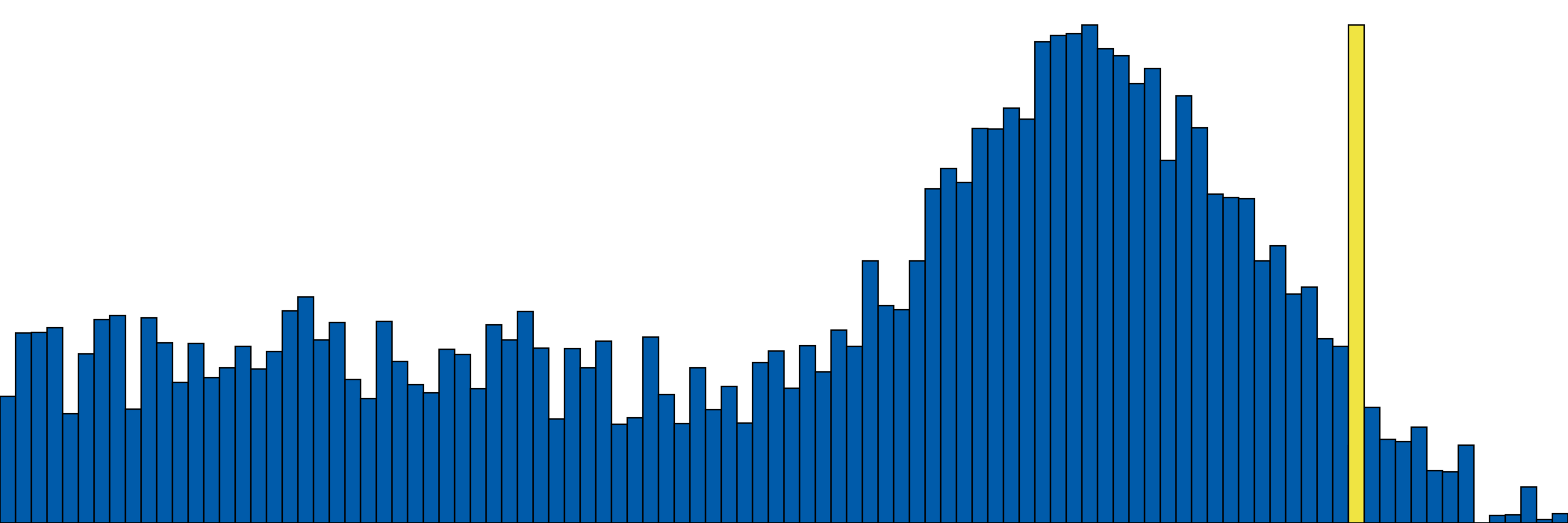
This helps so much with interpreting our interpretability measure! We can get a good idea of how strongly our result supports our hypothesis: if it falls fairly far out in the tail of the null distribution, we can be more confident that our hypothesis is true. Follow-up tests could be informed by this result, as typical science operates.
However, it is possible that not just this part $A$ of $f$ is performing this function, and even that other parts of $f$ (maybe $B, A^\prime, \ldots$) are performing it better! With a different perspective (null hypothesis space), we might observe and conclude something completely different:
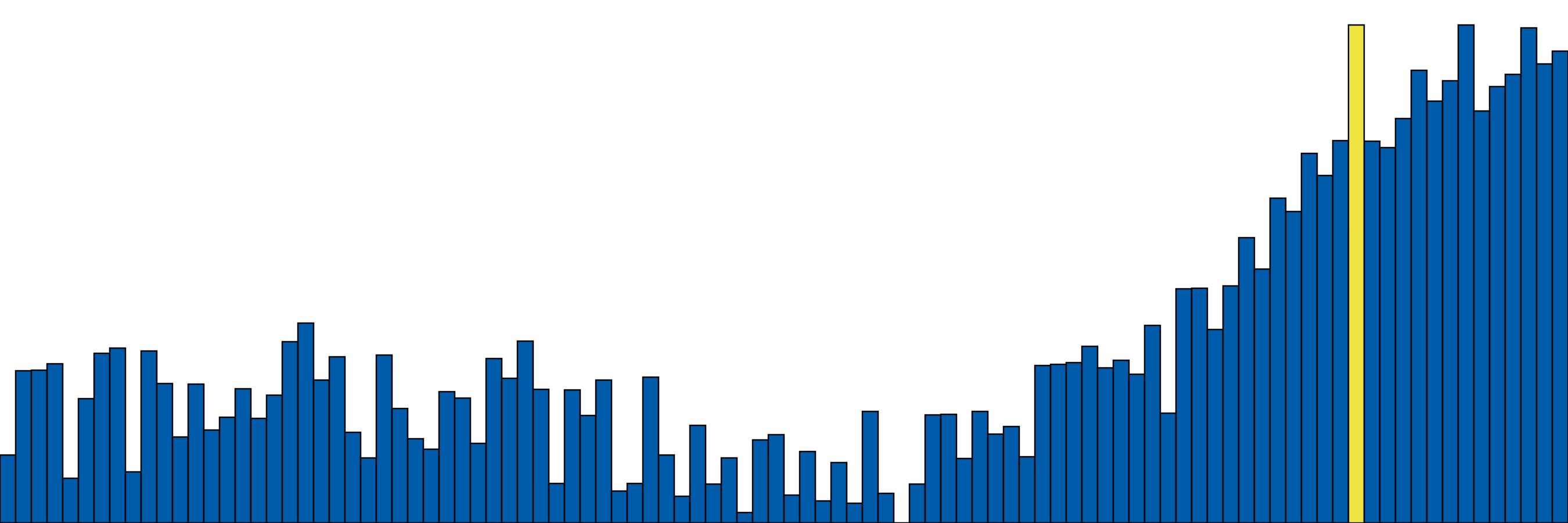
We have to decide the hypothesis space that corresponds to our specific interpretability question. Do we want to know if this part of the model is performing a particular function better than any other function? Or is it better than any other part of the model? Or maybe just better than any other part of the model on a particular subset of the data or sub-task? Choosing this question determines the hypothesis spaces, the types of samples we would draw, and the measures we would use to compare them. All of these form the definition of our hypothesis test.
It’s So Much Easier Than Real-World Science
In the real world we can never hope to draw enough samples to estimate complex, high-dimensional distributions. Costs of sample collection and computation can become exorbitant, e.g., computing summary statistics over functional MRI sequences. These can limit the number of potential tests that can be actually considered. But in our machine learning, neural network case we are only limited by our compute, and our compute only consists of possible paths through the model!
Again, if we really wanted to, we could enumerate all possible hypotheses for questions like “Which part of my model is responsible for behavior $A$?” In practice we would never do this and the compute cost can easily become obscene.2 But this does suggest that we do not have to worry about permutation costs in the same way that classical science does. We are not limited by ethical concerns of additional animal testing, or prohibitive costs associated with high-fidelity data collection or expert time, or the time it takes to run a physical experiment.
Even moreso, this type of testing is fully and embarrassingly parallel! Anyone with a specific hypothesis about a particular part of a network can test it, and that particular result, even if it turns out to be nothing, can be used as a sample for someone else’s null distribution if it is relevant to their hypothesis. We don’t even have to be careful about defining the hypothesis spaces at the start. We can collect any number of samples of the form “replace subset of model with my guess $g$ and measure loss”, and later define our hypothesis space to determine if a particular guess of a particular model subset is performing a particular function. A new subset can be tested, a new function could be replaced, and we can continuously compare subsequent measures against our growing null distribution, sliced to represent the specific null for that particular question.
As science progresses in the real world, our null distribution and suggested hypotheses can become better and better. In the same way we may identify a bimodal distribution over the Vitamin C we measure in apples and conclude that perhaps we should stratify by variety, we may find our original subgraph size is too fine-grained, or too general, or our function space too large, or too small. In this framing, failures are still extremely valuable, as they increase our confidence that successes are true successes. We can adjust our hypotheses as we learn from previous tests (in another language, slowly “recover more loss”).
Some More Concise and Concrete Research Directions
On the slightly more theoretical side, we should be able to come up with formalisms for defining hypothesis spaces and measures that are relevant to interpretability. We should be able to come up with a way to describe spaces of functions and ways to practically sample from them, for typical types of interpretability hypothesis tests. I don’t expect this to go all the way to things analogous to “minimax optimal uniformly most powerful” type results a la classical stats, but there is probably a cool medium between that and the current state of interpretability research. Perhaps some sub-topics under high-dimensional statistics could play larger roles.
On the more practical side, there are a lot tools that probably can be adapted or easily built to help with testing these hypotheses. Existing mechanistic interpretability tools are probably sufficient for the actual sampling and measure computation, but there are probably 1) automated systems that can help with the permutation testing schemes and 2) some sort of distributed or centralized hypothesis sharing and aggregation platforms that can help replicating existing tests and minimizing duplicate effort.
Minimally, it’s probably valuable to at least try to instantiate something like this against an existing interpretability result, e.g., if you sampled tons of functions “around” e.g., induction heads, and found that the original hypothesis was not supported, that would be a valuable standalone result.
Further Out
Optimistically, if everything works out, there I imagine a distributed hypothesis testing setup where individual researchers testing particular models for particular functions contribute their results to build out the “global null”. Slowly, we would build up a picture of what parts of what models are doing what, and how well they are doing it. Each “hypothesis” is connected to specific models, functions, samples, networks, and measures, and different slicing can result in different types of tests.
Say one organization tests a large number of different subgraphs, trying to identify which are important for induction. Say another organization tests a large number of different functions, trying to identify which function a particular subgraph is performing. The current model with its current subgraph and function represent the intersection of these two hypothesis spaces, and the results of these tests can be used to inform future tests in either space! Slowly, cooperation would build up a picture of what parts of what models are doing what, and how well they are doing it. None of the samples would be wasted, and as parts of “potential null distributions for future testing” get filled in from “more immediate need testing”, the “global null distribution” naturally grows to fully represent the space of possible hypotheses.
Yes, the space is impossible to enumerate, and we’ll never be able to test all possible hypotheses. But this is true of the real world too, and look how far we’ve come! Something is better than nothing, and I think this is a pretty good something.
Related Ideas and Directions
Fun With Measures
The cool thing about this is we don’t have to just use loss, or mean squared error, or any other typical measure. These may not capture exactly what we want to know. For networks the “acyclic directed graph” part is important structure, and we can use measures that respect that structure. We can even bring in probabilistic and causal measures in some form.
These measures can become quite complex. Going back a bit, an interpretation of the statement “important for” can be seen as “dependent on”, suggesting either direct causality or a less strong conditional dependence. Practical measures that extend correlation metrics exist for independence and conditional independence (e.g., conditional mutual information, CODEC, etc.), and these can be used to decide if a particular part of a model is necessary for another’s function.
Informing Progressive Testing
Even if we ignore traditional statistical rigor, we can just get a better idea of different directions to explore: Our search for hypotheses can be informed, building on methods for things like Automated Circuit Discovery. If our goal is to just figure out “what is this thing”, we can inform our sampling using some sort of exploration/exploitation tradeoff: randomly sample “around” the current function or subgraph, find the most interesting samples, and then sample more around those. (Don’t throw out the samples that don’t support the hypothesis: they can be used to inform other, future tests!) We’re just narrowing our search space to more likely hypotheses.
Footnotes
-
With nice distributions, we have strong guarantees via the statistical test we choose (e.g., Z-Test) that our sample mean will not be too far from the true population mean if we have enough samples. ↩
-
I could potentially see some value in actually doing enumeration on small models, e.g., GPT-2. To get better handles on methods and measures. Results here could be used to inform sampling required for larger models, or even to narrow hypothesis selection for larger models. ↩